프로그래밍/파이썬 Python
Pandas 라이브러리 관련 함수 정리
한별요
2022. 1. 11. 00:59
파이썬으로 머신러닝을 다루다 보면 이렇게 데이터프레임을 많이 다루는데 매일 찾아보기도 귀찮고 해서
데이터 추가, 행 검색, 중복 검색, 상관관계... 등등 자주쓰는 함수들을 정리하였다.
위 ipynb파일을 열면 더 깔끔하게 확인할 수 있다.
In [201]:
import re, json
import pandas as pd
import numpy as np
import os

import matplotlib.pyplot as plt
import seaborn as sns
%matplotlib inline
In [202]:
PATH = 'data/'
In [203]:
AGE_GENDER = 'age_gender_bkts.csv'
COUNTRIY = 'countries.csv'
SESSIONS = 'sessions.csv'

TRAIN_USERS = 'train_users.csv'
TEST_USERS = 'test_users.csv'

SAMPLE = 'sample_submission_NDF.csv'
In [204]:
age_df = pd.read_csv(PATH + AGE_GENDER)
country_df = pd.read_csv(PATH + COUNTRIY)
session_df = pd.read_csv(PATH + SESSIONS)

train_df = pd.read_csv(PATH + TRAIN_USERS)
test_df = pd.read_csv(PATH + TEST_USERS)

sample_df = pd.read_csv(PATH + SAMPLE)
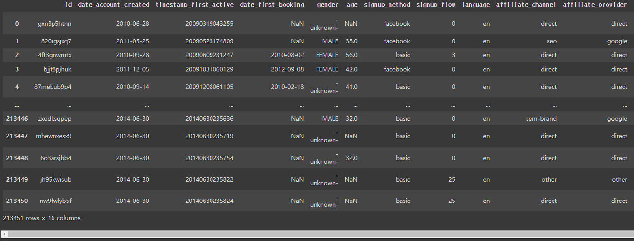
In [205]:
train_df
Out[205]:
1 데이터 분석
1.1 데이터 값 종류
In [206]:
train_df['country_destination'].unique()
Out[206]:
1.2 데이터 요약통계
In [207]:
train_df.describe()
Out[207]:
In [208]:
train_df.age.mean() # train_df['age'].mean()
Out[208]:
1.3 데이터 값 분석
In [209]:
train_df['country_destination'].value_counts()
Out[209]:
1.4 null 데이터 확인
In [210]:
pd.isnull(train_df) #null이 아닌지 확인할때는 pd.notnull(obj)
Out[210]:
In [211]:
train_df['gender'].isna().sum() #gender에서 결측치 개수
Out[211]:
In [212]:
train_df.isna().sum()
Out[212]:
1.5 데이터 타입 확인
In [213]:
train_df.dtypes
Out[213]:
1.6 컬럼이름
In [214]:
#컬럼 이름 확인
train_df.columns
Out[214]:
In [215]:
#컬럼 이름으로 조회
train_df['country_destination']
Out[215]:
In [216]:
#여러 컬럼 조회
train_df[['age','gender']]
Out[216]:
In [217]:
#컬럼 조건 검색
train_df[(train_df['age']>10)&(train_df['gender']=='FEMALE')]
Out[217]:
1.7 인덱싱
In [218]:
# 행 인덱스
train_df.iloc[:5]
Out[218]:
In [219]:
train_df.loc[train_df['gender']=='FEMALE'] #이건 굳이 loc안써도 됨
Out[219]:
In [220]:
#행,열인덱스 loc[행,열]
train_df.loc[train_df['gender']=='FEMALE', 'age']
Out[220]:
In [221]:
train_df.loc[train_df['gender']=='FEMALE', ['age','gender']]
Out[221]:
1.8 데이터 분포
In [222]:
#하나의 컬럼 분포
train_df['gender'].hist(bins=50, width = 0.4, figsize= (5,5), facecolor = "#2E495E", edgecolor = (0,0,0))
Out[222]:

In [223]:
feat_train = train_df['first_affiliate_tracked'].value_counts()
fig = plt.figure(figsize=(8,4))
sns.set_palette("muted") #색 지정
sns.barplot(feat_train.index.values, feat_train.values)
plt.title('first_affiliate_tracked of training dataset')
plt.ylabel('Counts')
plt.tight_layout()

In [224]:
#두 열 간 분포 보기
plt.figure(figsize=(12, 8))
sns.countplot(x=train_df['first_affiliate_tracked'],
              hue='gender',
              data=train_df)
plt.xticks(rotation=45)
Out[224]:

In [225]:
#히트맵으로도 볼 수 있음
notndf = train_df[train_df['country_destination']!='NDF']
lang = notndf.groupby(['first_affiliate_tracked','country_destination']).id.count().reset_index()
plt.figure(figsize=(10,10))
fig = sns.heatmap(lang.pivot_table(values='id',index='first_affiliate_tracked',columns='country_destination',aggfunc='sum'), cmap='Reds')

In [226]:
#레이블 별 특징 분포 그래프
def plot_feature_by_label(dataframe, feature_name, label_name, title):
    try:
        print(feature_name)
        sns.set_style("whitegrid")
        ax = sns.FacetGrid(dataframe, hue=label_name,aspect=2.5)
        ax.map(sns.kdeplot,feature_name,shade=True)
        ax.set(xlim=(0, dataframe[feature_name].max()))
        ax.add_legend()
        ax.set_axis_labels(feature_name, 'proportion')
        ax.fig.suptitle(title)
        plt.show()
    except:
        print("skip")
        plt.show()
In [227]:
for feature_name in train_df.drop(['country_destination','id'],axis=1).keys():
    plot_feature_by_label(train_df, feature_name, 'country_destination', feature_name + ' vs country_destination')

#이번 같이 데이터값 대부분이 문자인 경우엔 잘 안됨
#x 데이터형이 [숫자, 날짜]중 하나로 치환되어야함!


In [ ]:
2 데이터 전처리
2.1 이상치를 특정 값으로
In [228]:
#결측치로 처리
train_df.loc[~train_df['age'].between(18, 100), 'age'] = np.nan
2.2 중복/누락 데이터 처리
In [229]:
#중복 행 조회
train_df.duplicated()
Out[229]:
In [230]:
#중복 행 제거
train_df = train_df.drop_duplicates()
In [231]:
#누락 데이터 제거
train_df = train_df.dropna()
In [232]:
#누락 데이터 채우기
train_df = train_df.fillna(0) #0으로 채워짐
2.3 행&열 삭제
In [233]:
#drop 함수로 열 삭제
train_data = train_df.drop('id',axis=1) #행 삭제할 땐 axis=0
특정 열 값들 가져오기
In [234]:
genders = [x for x in train_df['gender']]
genders
Out[234]:
2.4 One-hot-encoding
In [235]:
cat_features = ['gender',  'first_browser']
for f in cat_features:
    data_dummy = pd.get_dummies(train_df[f], prefix=f) # encode categorical variables
    train_df.drop([f], axis=1, inplace = True) # drop encoded variables
    train_df = pd.concat((train_df, data_dummy), axis=1) # concat numerical and categorical variables

train_df
Out[235]:
2.5 시계열 데이터로 변환
In [236]:
train_df['date_account_created'] = pd.to_datetime(train_df['date_account_created'])
train_df['date_first_booking'] = pd.to_datetime(train_df['date_first_booking'])


date = train_df['date_account_created']
sub = train_df['date_first_booking'] - train_df['date_account_created']

import datetime
len([x for x in sub if x < datetime.timedelta(days=10)])
Out[236]:
2.6 특정 열 데이터 타입 변환
In [242]:
train_df['age'] = train_df['age'].astype(int)
train_df['age'].dtypes
Out[242]:
3 상관관계 분석
In [164]:
sns.heatmap(train_df.corr(), annot=True) #dtype이 수치형인것만 나오는거같음..
Out[164]:

In [165]:
train_df.corr()
Out[165]:
4 훈련/테스트 데이터 분리
4.1 레이블 분리
In [166]:
X, y = train_df.drop('country_destination',axis= 1), train_df['country_destination']
4.2 데이터 분할
In [167]:
from sklearn.model_selection import train_test_split # 데이터 셋 분할

X_train, X_test, y_train, y_test = train_test_split(X, y, test_size = 0.2, random_state = 42)
5 주성분 분석
데이터가 숫자로 되어있어야 해서 다른 데이터 사용 //url을 통해 데이터 다운
In [170]:
import requests

data = requests.get("https://archive.ics.uci.edu/ml/machine-learning-databases/breast-cancer-wisconsin/wdbc.data")
dataset_path = os.path.join('data', 'wdbc.data')
columns = [
    "diagnosis",
    "radius_mean", "texture_mean", "perimeter_mean", "area_mean", "smoothness_mean",
    "compactness_mean", "concavity_mean", "points_mean", "symmetry_mean", "dimension_mean",
    "radius_se", "texture_se", "perimeter_se", "area_se", "smoothness_se",
    "compactness_se", "concavity_se", "points_se", "symmetry_se", "dimension_se",
    "radius_worst", "texture_worst", "perimeter_worst", "area_worst", "smoothness_worst",
    "compactness_worst", "concavity_worst", "points_worst", "symmetry_worst", "dimension_worst",
    ]


with open(dataset_path, "w") as f:
  f.write(data.text)

dataset = pd.read_csv(dataset_path, names=columns)
dataset.sample(5)
X = dataset[dataset.columns[1:]]
dataset['target'] = (dataset['diagnosis']=='B')*0 + \
                   (dataset['diagnosis']=='M')*1
y = dataset['target']
X_train, X_test, Y_train, Y_test = train_test_split(X, y, test_size=0.25)
RFECV 실행
In [171]:
from sklearn.feature_selection import RFECV
from sklearn.tree import DecisionTreeClassifier
min_features_to_select = 1
clf = DecisionTreeClassifier(max_depth=2, min_samples_leaf=10, random_state=12)
rfe = RFECV(estimator = clf,
           step=1,
           cv=5,
           scoring='accuracy',
           min_features_to_select = min_features_to_select
           )
rfe = rfe.fit(X_train,Y_train)
특징 선택을 위한 훈련 과정의 성능 그래프
In [172]:
plt.figure(figsize=(7,5))
plt.xlabel("Number of features selected")
plt.ylabel("Cross validation score (# of correct classifications)")
plt.plot(range(min_features_to_select, len(rfe.grid_scores_)+min_features_to_select), rfe.grid_scores_)
plt.show()

위 사진을 보면 특징을 3개정도까지만 써도 충분한 정확도를 보여주고 그것보다 많은 특징을 썼을땐 성능을 그렇게 좌우하지 않는 걸 볼 수있음
선택된 특징 확인
In [173]:
best_features = X_train.columns.values[rfe.support_]
drop_features = [ column_name for column_name in columns[1:] if column_name not in best_features ]

print('Optimal number of features :', rfe.n_features_)
print('Best features :', best_features)
print('Drop features :', drop_features)
6 랜덤 포레스트
In [176]:
from sklearn.ensemble import RandomForestClassifier

clf = RandomForestClassifier(max_features=4,random_state=0)
clf.fit(X_train,Y_train)
print('Accuracy of Random Forest Classifier on training data: {:.2f}'.format(clf.score(X_train,Y_train)))
print('Accuracy of Random Forest Classifier on testing data: {:.2f}'.format(clf.score(X_test,Y_test)))
모델 평가
In [197]:
from sklearn.metrics import accuracy_score, confusion_matrix, classification_report
model = clf
prediction = model.predict(X_test)
cnf_matrix = confusion_matrix(Y_test, prediction)
cnf_matrix
Out[197]:
In [198]:
report = classification_report(Y_test, prediction)
print(report)
In [ ]: